10Python for Scientific Computing¶

10.1Overview¶

Python is the most popular language for many aspects of scientific computing.

This is due to

• the accessible and expressive nature of the language itself,

• the huge range of high quality scientific libraries,

• the fact that the language and libraries are open source,

• the central role that Python plays in data science, machine learning and AI.

In previous lectures, we used some scientific Python libraries, including NumPy and Matplotlib.

However, our main focus was the core Python language, rather than the libraries.

Now we turn to the scientific libraries and give them our full attention.

In this introductory lecture, we’ll discuss the following topics:

1. What are the main elements of the scientific Python ecosystem?

2. How do they fit together?

3. How is the situation changing over time?

In addition to what’s in Anaconda, this lecture will need

Let’s start with some imports:

10.2Major Scientific Libraries¶

Let’s briefly review Python’s scientific libraries.

10.2.1Why do we need them?¶

We need Python’s scientific libraries for two reasons:

1. Python is small

2. Python is slow

Python is small

Core python is small by design -- this helps with optimization, accessibility, and maintenance

Scientific libraries provide the routines we don’t want to -- and probably shouldn’t -- write ourselves

• numerical integration, interpolation, linear algebra, root finding, etc.

Python is slow

Another reason we need the scientific libraries is that pure Python is relatively slow.

Scientific libraries accelerate execution using three main strategies:

1. Vectorization: providing compiled machine code and interfaces that make this code accessible

2. JIT compilation: compilers that convert Python-like statements into fast machine code at runtime

3. Parallelization: Shifting tasks across multiple threads/ CPUs / GPUs /TPUs

We will discuss these ideas in depth below.

10.2.2Python’s Scientific Ecosystem¶

At QuantEcon, the scientific libraries we use most often are

• NumPy

• SciPy

• Matplotlib

• JAX

• Pandas

• Numba

Here’s how they fit together:

• NumPy forms foundations by providing a basic array data type (think of vectors and matrices) and functions for acting on these arrays (e.g., matrix multiplication).

• SciPy builds on NumPy by adding numerical methods routinely used in science (interpolation, optimization, root finding, etc.).

• Matplotlib is used to generate figures, with a focus on plotting data stored in NumPy arrays.

• JAX includes array processing operations similar to NumPy, automatic differentiation, a parallelization-centric just-in-time compiler, and automated integration with hardware accelerators such as GPUs.

• Pandas provides types and functions for manipulating data.

• Numba provides a just-in-time compiler that plays well with NumPy and helps accelerate Python code.

We will discuss all of these libraries at length in this lecture series.

10.3Why is Pure Python Slow?¶

As mentioned above, numerical code written in pure Python is relatively slow.

Let’s try to understand what’s driving slow execution speeds.

10.3.1Type Checking¶

One source of overhead in pure Python operations is type checking.

Let’s try to understand the issues.

10.3.1.1Dynamic typing¶

Consider this Python operation

Even for this simple operation, the Python interpreter has a fair bit of work to do.

For example, in the statement a + b, the interpreter has to know which operation to invoke.

If a and b are strings, then a + b requires string concatenation

If a and b are lists, then a + b requires list concatenation

As a result, when executing a + b, Python must first check the type of the objects and then call the correct operation.

This involves overhead.

If we repeatedly execute this expression in a tight loop, the overhead becomes large.

10.3.1.2Static types¶

Compiled languages avoid these overheads with explicit, static types.

For example, consider the following C code, which sums the integers from 1 to 10

#include <stdio.h>

int main(void) {
    int i;
    int sum = 0;
    for (i = 1; i <= 10; i++) {
        sum = sum + i;
    }
    printf("sum = %d\n", sum);
    return 0;
}

The variables i and sum are explicitly declared to be integers.

Moreover, when we make a statement such as int i, we are making a promise to the compiler that i will always be an integer, throughout execution of the program.

As such, the meaning of addition in the expression sum + i is completely unambiguous.

There is no need for type-checking and hence no overhead.

10.3.2Data Access¶

Another drag on speed for high-level languages is data access.

To illustrate, let’s consider the problem of summing some data --- say, a collection of integers.

10.3.2.1Summing with Compiled Code¶

In C or Fortran, an array of integers is stored in a single contiguous block of memory

• For example, a 64 bit integer is stored in 8 bytes of memory.

• An array of $n$ such integers occupies $8n$ consecutive bytes.

Moreover, the data type is known at compile time.

Hence, each successive data point can be accessed by shifting forward in memory space by a known and fixed amount.

10.3.2.2Summing in Pure Python¶

Python tries to replicate these ideas to some degree.

For example, in the standard Python implementation (CPython), list elements are placed in memory locations that are in a sense contiguous.

However, these list elements are more like pointers to data rather than actual data.

Hence, there is still overhead involved in accessing the data values themselves.

Such overhead is a major culprit when it comes to slow execution.

10.3.3Summary¶

Does the discussion above mean that we should just switch to C or Fortran for everything?

The answer is: Definitely not!

For any given program, relatively few lines are ever going to be time-critical.

Hence it is far more efficient to write most of our code in a high productivity language like Python.

Moreover, even for those lines of code that are time-critical, we can now equal or outpace binaries compiled from C or Fortran by using Python’s scientific libraries.

On that note, we emphasize that, in the last few years, accelerating code has become essentially synonymous with parallelization.

This task is best left to specialized compilers!

10.4Accelerating Python¶

In this section we look at three related techniques for accelerating Python code.

Here we’ll focus on the fundamental ideas.

Later we’ll look at specific libraries and how they implement these ideas.

10.4.1Vectorization ¶

One method for avoiding memory traffic and type checking is array programming.

Many economists usually refer to array programming as “vectorization.”

The key idea is to send array processing operations in batch to pre-compiled and efficient native machine code.

The machine code itself is typically compiled from carefully optimized C or Fortran.

For example, when working in a high level language, the operation of inverting a large matrix can be subcontracted to efficient machine code that is pre-compiled for this purpose and supplied to users as part of a package.

The core benefits are

1. type-checking is paid per array, rather than per element, and

2. arrays containing elements with the same data type are efficient in terms of memory access.

The idea of vectorization dates back to MATLAB, which uses vectorization extensively.

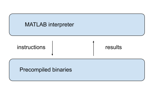
NumPy uses a similar model, inspired by MATLAB

10.4.2Vectorization vs pure Python loops¶

Let’s try a quick speed comparison to illustrate how vectorization can accelerate code.

Here’s some non-vectorized code, which uses a native Python loop to generate, square and then sum a large number of random variables:

The following vectorized code uses NumPy, which we’ll soon investigate in depth, to achieve the same thing.

As you can see, the second code block runs much faster.

It breaks the loop down into three basic operations

1. draw n uniforms

2. square them

3. sum them

These are sent as batch operators to optimized machine code.

10.4.3JIT compilers¶

At best, vectorization yields fast, simple code.

However, it’s not without disadvantages.

One issue is that it can be highly memory-intensive.

This is because vectorization tends to create many intermediate arrays before producing the final calculation.

Another issue is that not all algorithms can be vectorized.

Because of these issues, most high performance computing is moving away from traditional vectorization and towards the use of just-in-time compilers.

In later lectures in this series, we will learn about how modern Python libraries exploit just-in-time compilers to generate fast, efficient, parallelized machine code.

10.5Parallelization¶

The growth of CPU clock speed (i.e., the speed at which a single chain of logic can be run) has slowed dramatically in recent years.

Chip designers and computer programmers have responded to the slowdown by seeking a different path to fast execution: parallelization.

This involves

1. increasing the number of CPUs embedded in each machine

2. connecting hardware accelerators such as GPUs and TPUs

For programmers, the challenge has been to exploit this hardware running many processes in parallel.

Below we discuss parallelization for scientific computing, with a focus on

1. tools for parallelization in Python and

2. how these tools can be applied to quantitative economic problems.

10.5.1Parallelization on CPUs¶

Let’s review the two main kinds of CPU-based parallelization commonly used in scientific computing and discuss their pros and cons.

10.5.1.1Multithreading¶

Multithreading means running multiple threads of execution within a single process.

All threads share the same memory space, so they can read from and write to the same arrays without copying data.

For example, when a numerical operation on a large array runs on a modern laptop, the workload can be split across the machine’s multiple CPU cores, with each core handling a portion of the array.

10.5.1.2Multiprocessing¶

Multiprocessing means running multiple independent processes, each with its own separate memory space.

Because memory is not shared, processes communicate by passing data between them.

Multiprocessing can run on a single machine or be distributed across a cluster of machines connected by a network.

10.5.1.3Which Should We Use?¶

For numerical work on a single machine, multithreading is usually preferred --- it is lightweight and the shared memory model is very convenient.

Multiprocessing becomes important when scaling beyond a single machine.

For the great majority of what we do in these lectures, multithreading will suffice.

10.5.2Hardware Accelerators¶

A more dramatic source of parallelism comes from specialized hardware accelerators, particularly GPUs (Graphics Processing Units).

GPUs were originally designed for rendering graphics, which requires performing the same operation on many pixels simultaneously.

This architecture --- thousands of simple cores executing the same instruction on different data points --- turns out to be ideal for scientific computing.

When a computation can be expressed as independent operations on large arrays of data, GPUs can be orders of magnitude faster than CPUs.

TPUs (Tensor Processing Units), designed by Google for machine learning, follow a similar philosophy, optimizing for massive parallel matrix operations.

10.5.3Accessing GPU Resources¶

Many workstations and laptops now come with capable GPUs, and a single modern GPU is often sufficient for individual research projects.

Modern Python libraries like JAX, discussed extensively in this lecture series, automatically detect and use available GPUs with minimal code changes.

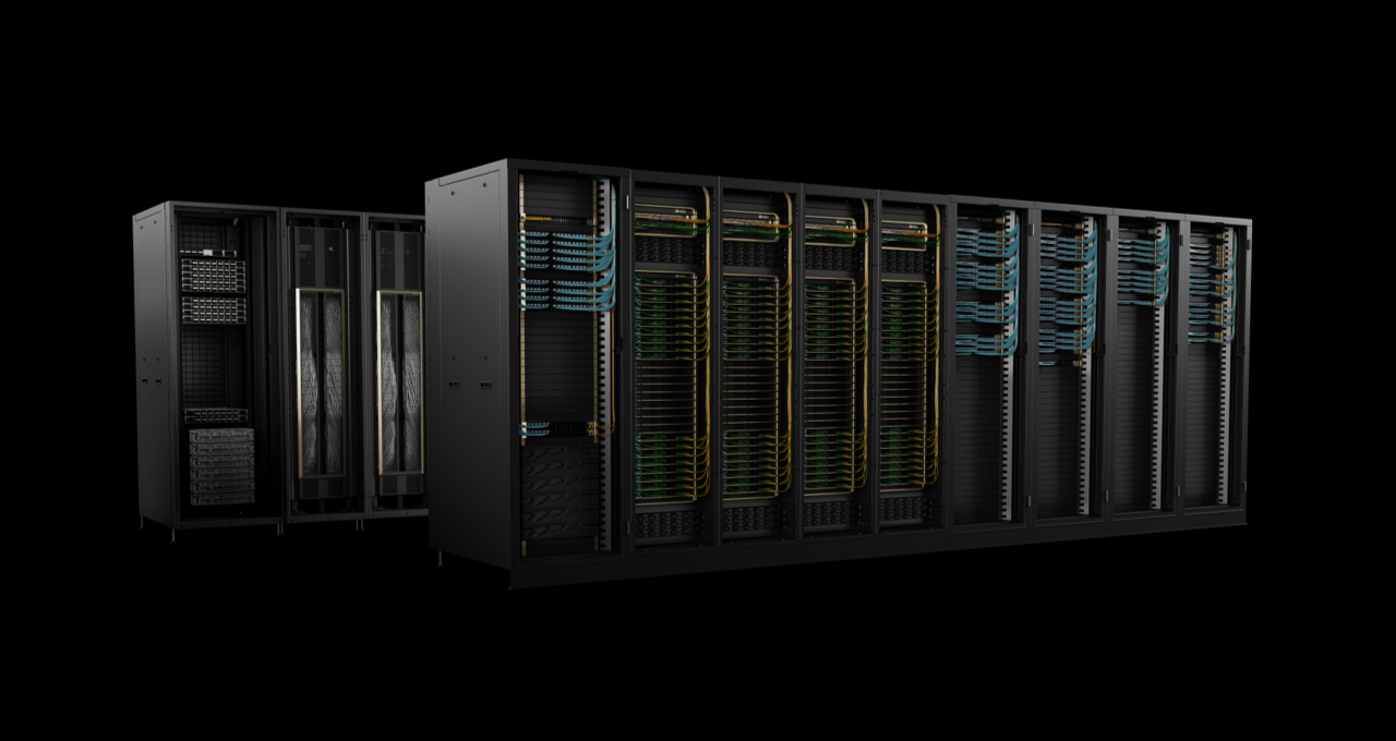
For larger-scale problems, multi-GPU servers (often 4--8 GPUs per machine) are increasingly common.

With appropriate software, computations can be distributed across multiple GPUs, either within a single server or across a cluster.

We will explore GPU computing in more detail in later lectures, applying it to a range of economic applications.